Hyperspectral AI for Industrial Applications

Table of Contents

Key Findings

Technical Overview

# Hyperspectral Processing Pipeline
def process_hyperspectral_cube(data_cube):
    # Noise reduction using adaptive filtering
    filtered_cube = adaptive_spectral_filter(data_cube)
    
    # Atmospheric correction and normalization
    corrected_cube = atmospheric_correction(filtered_cube)
    
    # Feature extraction using deep learning
    features = spectral_cnn_extractor(corrected_cube)
    
    # Classification and anomaly detection
    results = classify_materials(features)
    
    return results
                                

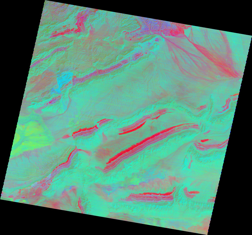
Hyperspectral AI: From Photons to Decisions

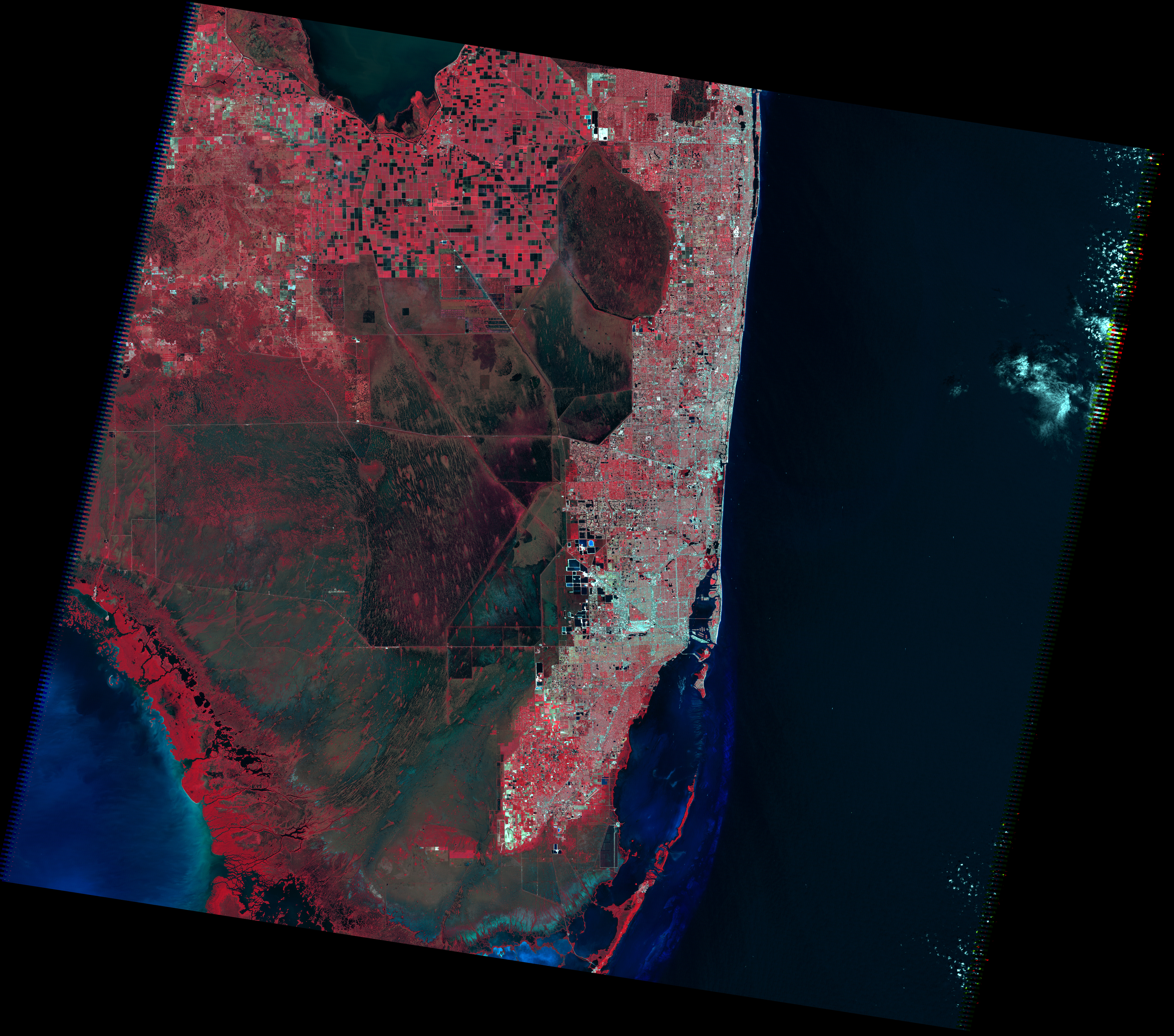
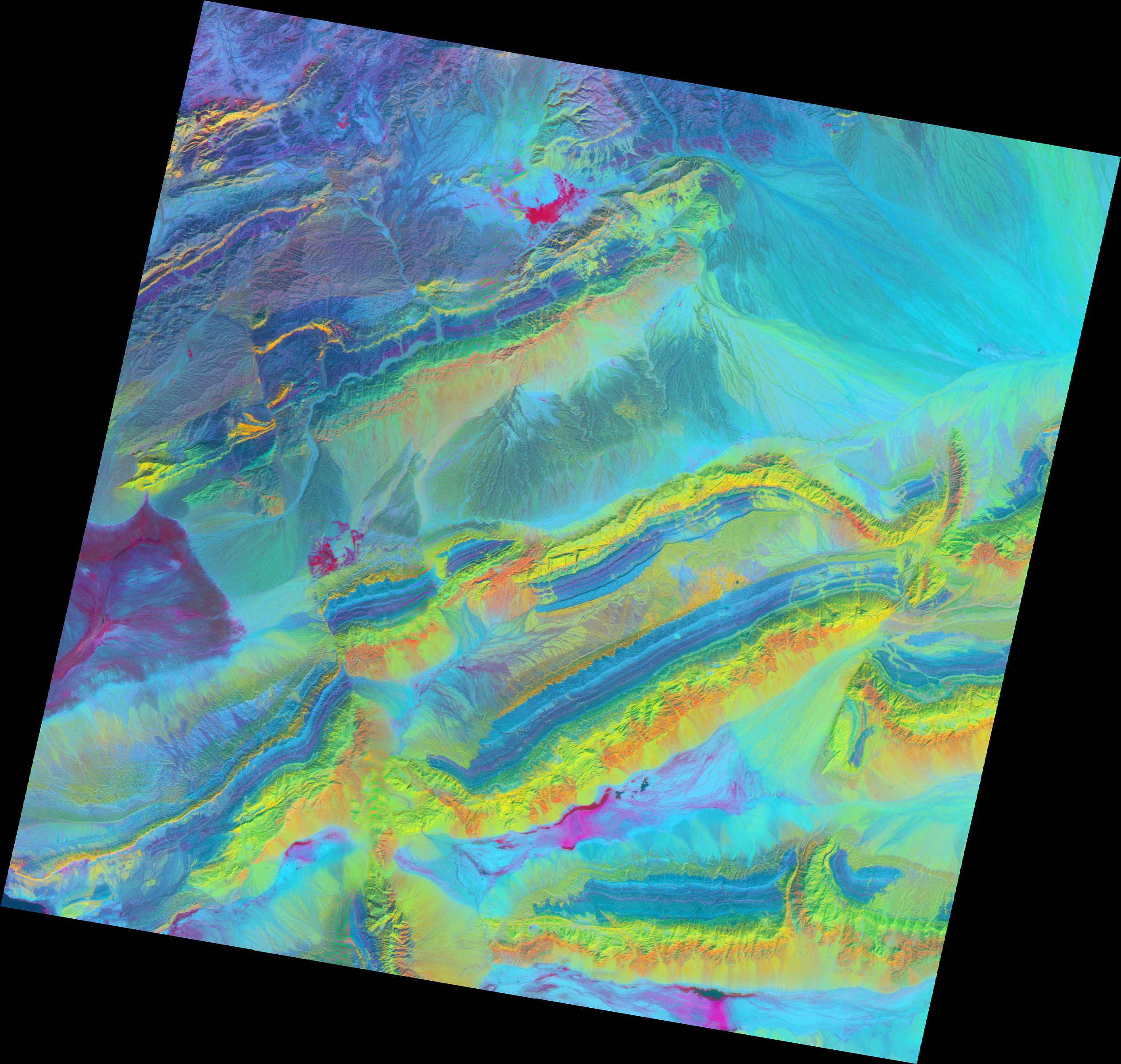
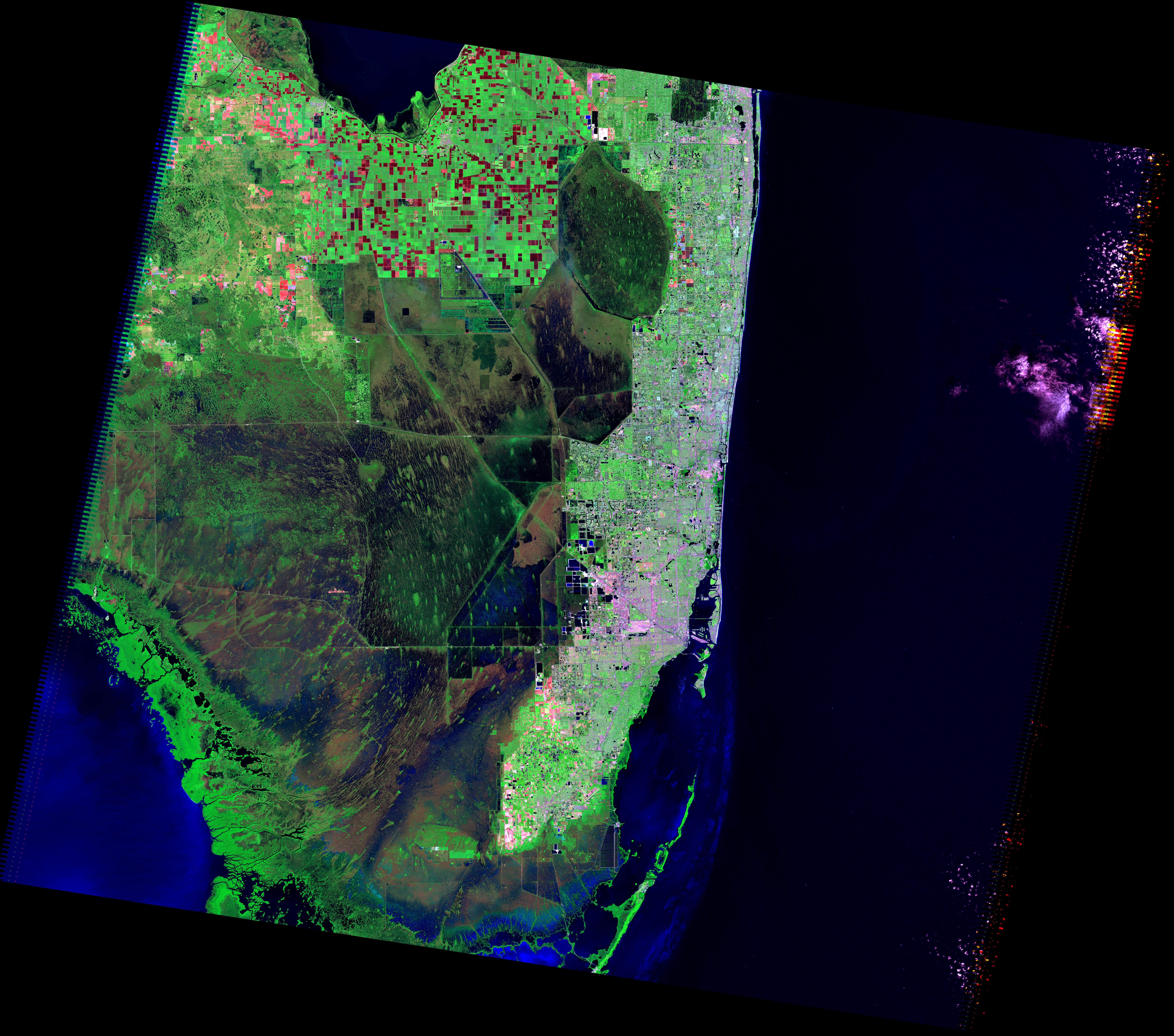
Hyperspectral imaging captures hundreds of contiguous spectral bands per pixel, enabling material identification and anomaly detection that far exceed RGB. When fused with modern deep learning, it unlocks powerful, real-time industrial systems. Below is a short explainer video, followed by a gallery of spectral composites and application examples.

Florida 432 Piqiang 468 Piqiang NIR

Industrial Applications

A Practical Guide to Hyperspectral AI in Industry

Hyperspectral imaging (HSI) systems measure reflected or emitted light across tens to hundreds of narrow, contiguous spectral bands. Unlike RGB, which compresses spectral nuance into just three channels, HSI produces a data cube: X and Y are spatial dimensions, and the Z-axis carries spectral intensity across wavelengths. This richer signal makes subtle material differences legible—coatings, contaminants, moisture, grain alignment, mineralogy, and chemical composition—which is why HSI is increasingly central to quality control, sorting, and non-destructive evaluation. When integrated with well-designed AI models and real-time pipelines, HSI becomes a practical, robust tool for the factory floor.

In this article, we translate state-of-the-art research and field experience into an actionable blueprint for deploying HSI + AI systems. We outline how to select optics and sensors, engineer lighting, build efficient data pipelines, train models that generalize, and validate performance against production constraints such as takt time and uptime. We also link to peer-reviewed literature for deeper reading (see References). To keep this practical, we highlight failure modes, guardrails, and the economics that determine whether a pilot becomes a production win.

The guiding principle is simple: optimize the whole system, not just the model. Spectral performance without illumination stability is brittle. Edge throughput without a labeling plan yields poor decisions. And models that excel on single-lot datasets can fail when suppliers or fixtures change. Success with HSI blends physics, engineering, data, and operations into one coherent workflow.

1) Hardware Fundamentals

An HSI system consists of an imaging spectrometer, optics, illumination, motion/scan mechanics (if required), and compute. Common modalities include pushbroom (line-scan) spectrometers for conveyor applications, and snapshot arrays for static scenes. Key levers:

• Spectral range: VNIR (400–1000 nm) captures visible and near-infrared; SWIR (1000–2500 nm) resolves moisture, polymers, and organics; MWIR/LWIR enable thermal emissivity studies.
• Spectral resolution: Narrower bands increase separability but raise noise; tune to application-specific signatures and SNR.
• Optics and F/#: Throughput affects exposure; aberrations and stray light impact calibration and downstream model performance.
• Illumination geometry: Uniform, stable lighting is non-negotiable; use line lights for pushbroom, integrate diffusers to minimize specular highlights.
• Motion control: In pushbroom systems, conveyor speed and line rate must match to avoid aspect ratio distortion and ensure consistent per-pixel dwell time.

Practical hint: If you’re new to HSI, start with VNIR on a controlled line. Validate SNR and class separability before scaling spectral range. Many projects stall not on algorithms, but on lighting and fixture stability. A 2% drift in intensity or angle can erase margins that your classifier depends on.

Choosing between pushbroom and snapshot modalities depends on scene dynamics. Pushbroom excels on moving targets with consistent motion (web materials, conveyors). Snapshot sensors simplify mechanics for static or slow scenes, at the cost of per-band SNR and sometimes spatial resolution. If you must scan, prioritize mechanical rigidity, vibration isolation, and encoder integration—the best models can’t rescue smeared data.

2) Calibration and Preprocessing

Raw HSI data cubes require careful calibration to remove system and environmental effects. A standard workflow includes dark current subtraction, white reference normalization (to convert to reflectance), stray light correction, and wavelength registration. For production lines, schedule automated white/dark cycles and monitor calibration metrics over time.

• Automate dark/white captures during shift changes or when the line idles to minimize disruption.
• Log illumination temperature and intensity; compensate or alert when drift exceeds thresholds.
• Quantize and compress data with care; preserve spectral fidelity for downstream models.

Preprocessing also includes denoising (e.g., Savitzky–Golay filtering), baseline correction, and dimensionality reduction. While PCA/ICA are classic tools, modern approaches learn spectral embeddings jointly with the task model, often outperforming handcrafted pipelines in varying conditions.

Treat calibration as a monitored service. Track white-reference histograms, per-band SNR, and wavelength alignment using known spectral features. Version your calibration artifacts so you can reproduce decisions and audit changes. When anomalies appear in production, nine times out of ten the root cause lies upstream of the model—and calibration logs tell the story.

3) Labeling and Dataset Design

Building a representative dataset is the most important predictor of success. For classification or segmentation, curate examples across the true distribution of materials, suppliers, and environmental conditions. Explicitly include borderline cases and expected drift: new suppliers, slightly different coatings, aging fixtures, sensor re-calibrations.

• Define classes by decision intent (e.g., accept/reject) rather than material taxonomy when appropriate; this simplifies downstream operations.
• Capture paired RGB + HSI when possible; RGB aids annotation and debugging, and can serve as a fallback modality.
• Use spectral regions-of-interest (ROIs) for faster labeling; don’t annotate every pixel if area labels suffice for your KPI.

For rare defects, deploy a conservative model in shadow mode to flag uncertain regions for review. Over time, you’ll concentrate labeling effort on decision boundaries where it matters most. Stratify by lot and time; a model that performs well within-lot but poorly across-lot isn’t production-ready.

4) Model Architectures that Work

Effective models exploit both spectral and spatial structure. Three patterns are prevalent:

1. 1D spectral networks operate along the spectral axis per pixel, enabling fast, low-parameter classifiers for homogeneous scenes.
2. 2D CNNs on composite bands (e.g., choose 8–16 informative bands) balance speed with spatial context.
3. 3D CNNs/transformers jointly model spectra and spatial neighborhoods, yielding top accuracy when compute allows.

In production, hybrid strategies excel: a lightweight 1D spectral gate routes ambiguous regions to a heavier 3D model, preserving throughput. Temporal smoothing with causal filters reduces flicker in decisions.

Self-supervised pretraining on unlabeled cubes can dramatically reduce labeled data requirements. Contrastive methods that treat neighboring spectra as positives and distant spectra as negatives build robust embeddings. Physics-informed networks that encode smoothness and known absorption features further stabilize predictions under lighting drift.

5) Real-Time Inference and Edge Compute

Line rates impose tight budgets. Aim for sub-50 ms end-to-end latency per frame region. Techniques that help:

• Quantize models to INT8 with careful calibration; validate spectral sensitivity post-quantization.
• Use CUDA graphs and fused kernels to minimize overhead.
• Tessellate the scene; process ROIs prioritized by motion and prior detections.
• Cache per-material spectral templates and enable early exits when matches are confident.

Architecturally, separate acquisition from inference and decision threads with lock-free queues. Handle backpressure gracefully—if the model can’t keep up, degrade (larger stride, band selection, or route to a faster fallback) rather than dropping frames blindly. Expose health metrics—frame rate, queue depth, GPU memory, per-band SNR—to your HMI/SCADA.

6) Validation, KPIs, and Operations

Define KPIs in operational terms (FPY, ppb defect rate, yield, scrap cost) and measure on blind runs. Include:

• Confusion matrices by material and lot
• ROC/PR curves for threshold tuning under cost asymmetry
• MTBF/MTTR for the full system (camera, lighting, compute)
• Uptime, takt time impact, and operator interventions

Close the loop with root-cause analysis: when misclassifications occur, correlate with sensor logs (temperature, exposure), lighting drift, and asset changes. Maintain a golden-set replay harness to regression-test models before deployment.

Validation isn’t a one-off event; schedule periodic drift audits replaying fresh data through current and prior models. Track calibration deltas and model retrain cadence. Treat updates like any other change-controlled process on the line, with rollbacks and sign-offs.

7) Economics and Scale-Up

The ROI case for HSI+AI depends on throughput, scrap reduction, labor reallocation, and avoided recalls. Start with a narrow, high-value defect or sorting use case; add classes once the pipeline is stable. Treat optics and lighting as capex with multi-year lifespan; model compute and maintenance as opex. Ensure your vendor contracts specify replacement SLAs for lighting and sensors.

A practical value ladder: Phase 1—install and calibrate; prove detectability on golden/defect sets. Phase 2—shadow mode on the live line; quantify false alarms and misses with operator feedback. Phase 3—closed-loop interventions (rejectors or robot pick) with guarded thresholds. Phase 4—broaden classes and integrate with MES/ERP for traceability. Gate each phase with KPI-based exit criteria.

8) Common Failure Modes

• Overfitting to one supplier or lot; fix with diversified sampling and domain randomization.
• Ignoring polarization and BRDF effects; fix with lighting geometry controls and cross-polarized setups.
• Data drift from lens fouling; add automated lens checks and cleaning SOPs.
• Misaligned conveyor speed and line rate; calibrate and monitor continuously.

Beware of conflating chemical sameness with spectral sameness. Two coatings with the same formulation can yield different spectra due to curing or surface roughness; different chemistries can look similar under certain lighting. Always validate separability under your exact illumination and view geometry.

9) Roadmap: From Pilot to Fleet

Bake in remote telemetry, configuration management, and A/B model rollout from day one. Use containerized deployments with health probes and automated fallbacks to a stable baseline. Document playbooks for recalibration and edge-node swap-out.

Fleet operations thrive on standardization. Normalize device configs (exposure, gain, line rate), directory structures, and metadata schemas. Implement over-the-air updates with cryptographic signing. Mirror logs and calibration artifacts to a central data lake for cross-site analytics and fleet-wide drift detection.

10) Where Research Meets Reality

The scientific literature on HSI is vast, spanning materials science, remote sensing, and computer vision. Contemporary studies explore transformers for spectral-context fusion, self-supervised pretraining on unlabeled cubes, and physics-informed networks that embed radiative transfer constraints. Industrialization means converting these ideas into stable, maintainable pipelines that run 24/7 on imperfect hardware. Use research to inform your design choices, then validate rigorously on your line.

For instance, remote-sensing methods such as vegetation indices and decorrelation stretches inspire industrial detection of organic residues or moisture gradients. The translation step is engineering—matching spectral regions to your illumination, mitigating motion blur, and ensuring compute budgets meet takt-time constraints.

Florida 742 Decorrelated Video Demo

Note: YouTube URLs are placeholders; replace with your channel’s videos. All local images and videos reference assets in this repository.

Use Cases and Case Snapshots

The following patterns appear across many deployments. Each snapshot focuses on lessons learned rather than exhaustive detail.

Metals and Foundry

Surface oxides, inclusions, and subtle alloy variations can be invisible in RGB yet distinct in VNIR/SWIR. A two-stage approach—fast spectral gating and 3D CNN refinement—enables early, precise rejection. Biggest wins came from stabilizing exposure near hot zones and maintaining clean enclosures.

Food and Agriculture

SWIR bands separate moisture and fats, enabling foreign object detection, grading, and ripeness estimation. Operator trust improved when overlays showed spectral evidence and model confidence alongside intuitive RGB views.

Polymers and Recycling

Sorting similar plastics requires spectral specificity under real-world contamination. Domain-randomized training improved generalization; economic gains emerged at scale as small per-piece lifts compounded.

Pharmaceuticals

Non-destructive checks for content uniformity and coating integrity demand controlled conditions and rigorous validation. Interpretability, audit trails, and change control are mandatory for regulated environments.

Governance, Safety, and Quality

Treat HSI as a quality instrument: document calibration SOPs, model change control, and operator training. Build fail-safes that default to manual inspection on confidence drops or calibration out-of-bounds. Involve quality and safety teams early to define acceptance criteria and traceability.

Deployment Patterns

• Inline: Real-time decisions with rejectors or robotic pick—highest constraints, largest payoffs.
• Nearline: Small buffers allow batching and higher-fidelity analysis—good for brownfield lines.
• Offline QA: Sampling-based deep dives—vital for model validation and vendor qualification.

FAQ

What if defects are rare? Use active learning and synthetic augmentations; start in shadow mode to accumulate borderline examples without disrupting production.

How many bands are enough? As many as needed to separate classes under your lighting and surface physics. Smart band selection often beats sheer band count.

Can this run on the edge? Yes—quantization, band selection, and hybrid routing enable real-time on compact GPUs/NPUs.

Summary

Hyperspectral AI succeeds when approached as a system problem. Nail the optics and fixtures, build representative datasets, deploy architectures matched to compute budgets, and validate continuously. Organizations that align quality engineering, operations, and data science realize durable gains: fewer defects, higher throughput, and deeper process insight.

Related Content

References

• Peer‑reviewed research on hyperspectral imaging and AI: Scientific Reports (Nature, 2024).
• NASA/USGS Landsat: landsat.gsfc.nasa.gov.
• Overview tutorials on industrial HSI lighting and optics (vendor-agnostic). Replace with your preferred training resources.